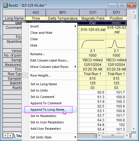
41 excel data labels from third column

stackoverflow.com › questions › 55735003Excel Pivot Table with multiple columns of data and each data ... Apr 17, 2019 · This will produce a Pivot Table with 3 rows. The first row will read Column Labels with a filter dropdown. The second row will read all the possible values of the column. The third row will be the count of each value in the above column. Repeat the process in the next available blank cell for the next category, which will produce something like ... Sharepoint excel data only showing column headers ... Data source is an excel file in sharepoint that is regularly being updated. No problem in connecting and accessing the file but when i view it in PBI desktop i can only see the 1st three rows. The 1st 2 rows are just merged rows for the file title and the actual data column headers are on the 3rd row. In PBI, no data from row 4 down is displayed.

peltiertech.com › excel-column-Excel Column Chart with Primary and Secondary Axes - Peltier ... Oct 28, 2013 · The second chart shows the plotted data for the X axis (column B) and data for the the two secondary series (blank and secondary, in columns E & F). I’ve added data labels above the bars with the series names, so you can see where the zero-height Blank bars are. The blanks in the first chart align with the bars in the second, and vice versa.

Excel data labels from third column

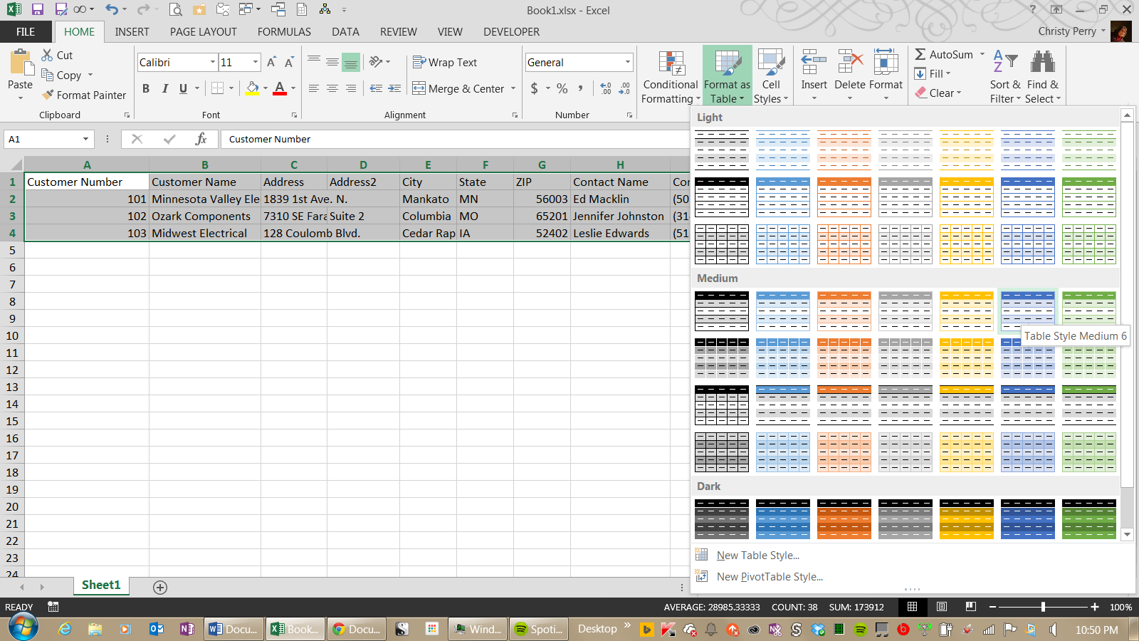
Match Two Columns in Excel and Return a Third (3 Ways ... In this article, we will see how to match two columns in Excel and return a third. In Excel, there are many find and match functions like FIND, MATCH, INDEX, VLOOKUP, HLOOKUP etc. Here in this article, we are going to use some of these. We will see some Excel formula to compare two columns and return a value. Click the icon in the content placeholder that will allow ... Go to Normal View (click the Normal button on the bottom right) and display Excel allows you to add chart elements —including chart titles, legends, and data labels —to make your chart easier to read. 3 - Click Download Visual. Use the Selection pane to manage objects in your document: re-order them, show or hide them, and group or ungroup ... Data Labels from Text Column using ... - Excel Help Forum I have a chart that draws from three columns: date, steps, and a notes field that provides a description of activities. The columns for date and steps have data in every cell but the notes field only has data in some cells. I use the notes field in the chart as the source for the chart's data labels.

Excel data labels from third column. › excel-stacked-column-chartStacked Column Chart in Excel (examples) - EDUCBA Overlapping of data labels, in some cases, this is seen that the data labels overlap each other, and this will make the data to be difficult to interpret. Things to Remember A stacked column chart in Excel can only be prepared when we have more than 1 data that has to be represented in a bar chart. Python 导出到 Excel | D栈 - Delft Stack 在上面的代码中，我们使用 Python 的 to_excel() 函数将 list1 和 list2 中的数据作为列导出到 sample_data.xlsx Excel 文件中。 我们首先将两个列表中的数据存储到 pandas DataFrame 中。之后，我们调用 to_excel() 函数并传递我们的输出文件和工作表的名称。 Add or remove data labels in a chart Right-click the data series or data label to display more data for, and then click Format Data Labels. Click Label Options and under Label Contains, select the Values From Cells checkbox. When the Data Label Range dialog box appears, go back to the spreadsheet and select the range for which you want the cell values to display as data labels. How can I add data labels from a third column to a ... Highlight the 3rd column range in the chart. Click the chart, and then click the Chart Layout tab. Under Labels, click Data Labels, and then in the upper part of the list, click the data label type that you want. Under Labels, click Data Labels, and then in the lower part of the list, click where ...

Can I add data labels from an unrelated column to a simple ... I would like to add data labels to the vertical chart representations with values from a third column. I am trying to show how many input/data points were included for each displayed column percentage (height) on the chart. The third column values range from 10-200, with an couple outliers up to 5,500, so a third axis doesn't display the data well. Apply Custom Data Labels to Charted Points - Peltier Tech Click once on a label to select the series of labels. Click again on a label to select just that specific label. Double click on the label to highlight the text of the label, or just click once to insert the cursor into the existing text. Type the text you want to display in the label, and press the Enter key. How to import an excel file with selected rows as column name? Now, in every sheet, the 3th row from top has a date value in MMM-YY (Jan-17) format in excel, and rest of the rows from 4 and below have numbers. I have to read last months data depending on which month I am executing my program, and I need the values from row 50 till the last. › filter-column-in-excelFilter Column in Excel (Example) | How To Filter a ... - EDUCBA Excel Column Filter (Table of Contents) Filter Column in Excel; How to Filter a Column in Excel? Filter Column in Excel. Filters in Excel are used for filtering the data by selecting the data type in the filter dropdown. By using a filter, we can make out the data that we want to see or on which we need to work.

Mac Excel 2008 - How to add Data Labels for Scatter Plot ... I have 3 columns of data: (A,B,C) Labels, X values, Y values When I select the Data Source for the Chart, there is a greyed out box for Category X axis labels, which is where I remember such information going in PC versions of Excel I used to use. From the formatting palette, the only options to select for labels add the values of column B, but I need the reference from column A. I'm not familiar with macros or visual basic. Can you please help me find a fix to add these labels? How to Use Cell Values for Excel Chart Labels Select the chart, choose the "Chart Elements" option, click the "Data Labels" arrow, and then "More Options.". Uncheck the "Value" box and check the "Value From Cells" box. Select cells C2:C6 to use for the data label range and then click the "OK" button. The values from these cells are now used for the chart data labels. Change the format of data labels in a chart Tip: To switch from custom text back to the pre-built data labels, click Reset Label Text under Label Options. To format data labels, select your chart, and then in the Chart Design tab, click Add Chart Element > Data Labels > More Data Label Options. Click Label Options and under Label Contains, pick the options you want. Guide: How to Name Column in Excel | Indeed.com The process of naming columns in Excel entails the steps described below: 1. Change the default column names Locate and open Microsoft Excel on your computer. Removing the actual header's name involves changing the first row of the column you intend to rename. Click inside the first row of the worksheet and insert a new row above the first one.

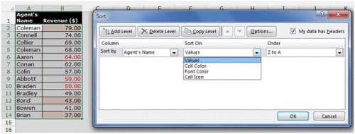
How to Sort data in Microsoft Excel

How to compare two columns and return values from the ... Then, select Look for a value in list option in the Choose a formula list box; And then, in the Arguments input text boxes, select the data range, criteria cell and column you want to return matched value from separately. 4. Then click Ok, and the first matched data based on a specific value has been returned.

Select data for a chart - Excel

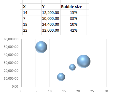
Excel VBA - Add Data Labels from Table body range - Stack ... Here's my final code inserting labels from the Table into the Bubble Chart: Sub DataLables() ActiveSheet.ChartObjects("Chart 1").Activate ActiveChart.FullSeriesCollection(1).DataLabels.Select For i = 1 To Range("Table1[Project '#]").Count ActiveChart.FullSeriesCollection(1).Points(i).DataLabel.Select Selection.Formula = Range("Table1[Project '#]").Cells(i, 1) Next i End Sub

How to add data labels from different column in an Excel chart?

Custom data labels in a chart - Get Digital Help You can easily change data labels in a chart. Select a single data label and enter a reference to a cell in the formula bar. You can also edit data labels, one by one, on the chart. With many data labels, the task becomes quickly boring and time-consuming. But wait, there is a third option using a duplicate series on a secondary axis.

Enable or Disable Excel Data Labels at the click of a button - How To - PakAccountants.com

› excel-line-column-chartLine Column Combo Chart Excel | Line Column Chart | Two Axes Creating a Line Column Combination Chart in Excel . You can create a combination chart in Excel but its cumbersome and takes several steps. Select your data and then click on the Insert Tab, Column Chart, 2-D Column. Note: Make sure your labels are formatted as text or they will be added to the chart as a third set of bars.

Merging 2 spreadsheets on Excel 2010 - Super User

peltiertech.com › text-labels-on-horizontal-axis-in-eText Labels on a Horizontal Bar Chart in Excel - Peltier Tech Dec 21, 2010 · In this tutorial I’ll show how to use a combination bar-column chart, in which the bars show the survey results and the columns provide the text labels for the horizontal axis. The steps are essentially the same in Excel 2007 and in Excel 2003. I’ll show the charts from Excel 2007, and the different dialogs for both where applicable.

How to Create Multi-Category Chart in Excel - Excel Board

Pulling Nonzero Values from a Column | MrExcel Message Board I have set up dummy formulas in column E to get a list like you described. To get the list shown in column G, follow these steps: 1. Ensure heading in col E 2. Set up F1:F2 as shown 3. Select column E by clicking its heading label. 4. Data|Filter|Advanced Filter...|Copy to another location|Criteria range: F1:F2|Copy to: G1|OK

How to edit the label of a chart in Excel? - Stack Overflow

How to add data labels from different column in an Excel ... This method will guide you to manually add a data label from a cell of different column at a time in an Excel chart. 1. Right click the data series in the chart, and select Add Data Labels > Add Data Labels from the context menu to add data labels. 2. Click any data label to select all data labels, and then click the specified data label to select it only in the chart.

How to Create Multi-Category Chart in Excel - Excel Board

› Automate-Reports-in-ExcelHow to Automate Reports in Excel (with Pictures) - wikiHow Apr 13, 2020 · Excel will track every click, keystroke, and formatting option you enter and add them to the macro's list. For example, to select data and create a chart out of it, you would highlight your data, click Insert at the top of the Excel window, click a chart type, click the chart format that you want to use, and edit the chart as needed.

Ease the Pain of Data Entry with an Excel Forms Template | Pryor Learning Solutions

Solved: Dataverse Edit data in Excel - Copy Data in One Te ... I am using the Dataverse "Edit data in Excel" feature as shown below. I have a Dataverse table that I need to copy the data in the Deal-Request-ID text col to the DRID lookup column which is currently blank for all rows. I just tried to copy and paste the data as shown below but I got the error, "...

How to create Custom Data Labels in Excel Charts - Efficiency 365

How to create Custom Data Labels in Excel Charts Create the chart as usual. Add default data labels. Click on each unwanted label (using slow double click) and delete it. Select each item where you want the custom label one at a time. Press F2 to move focus to the Formula editing box. Type the equal to sign. Now click on the cell which contains the appropriate label.

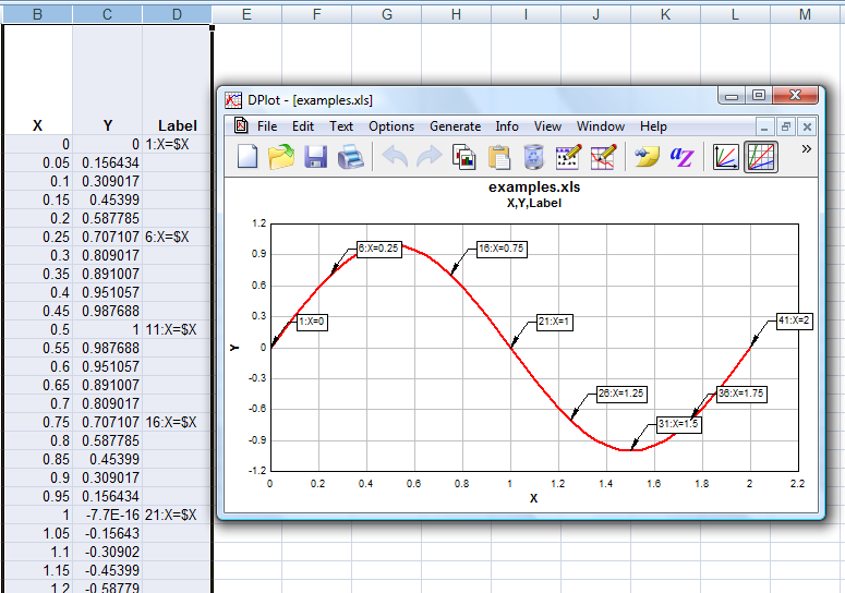
DPlot Windows software for Excel users to create presentation quality graphs

Prevent Overlapping Data Labels in Excel Charts - Peltier Tech Apply Data Labels to Charts on Active Sheet, and Correct Overlaps Can be called using Alt+F8 ApplySlopeChartDataLabelsToChart (cht As Chart) Apply Data Labels to Chart cht Called by other code, e.g., ApplySlopeChartDataLabelsToActiveChart FixTheseLabels (cht As Chart, iPoint As Long, LabelPosition As XlDataLabelPosition)

Label Columns In Excel - Ythoreccio

Pie Chart in Excel | How to Create Pie Chart | Step-by ... Step 1: Select the data to go to Insert, click on PIE, and select 3-D pie chart. Step 2: Now, it instantly creates the 3-D pie chart for you. Step 3: Right-click on the pie and select Add Data Labels. This will add all the values we are showing on the slices of the pie.

Change Column Colors / Show Percent Labels in Excel Column Chart

excel - VBA Change Data Labels on a Stacked Column chart ... Going into Excel, I select the chart I want to edit and then select all labels by going to Chart Tools > Add Chart Element > Data Labels > More Data Label Options Next I uncheck whatever options I don't want in my labels, and check those I do want, under the "Label Options" in the dialog I just opened.

How to Sort data in Microsoft Excel

Add Custom Labels to x-y Scatter plot in Excel ... Step 1: Select the Data, INSERT -> Recommended Charts -> Scatter chart (3 rd chart will be scatter chart) Let the plotted scatter chart be Step 2: Click the + symbol and add data labels by clicking it as shown below. Step 3: Now we need to add the flavor names to the label. Now right click on the label and click format data labels.

How to Create Multi-Category Chart in Excel - Excel Board

How to Print Labels From Excel? | Steps to Print Labels ... Navigate towards the folder where the excel file is stored in the Select Data Source pop-up window. Select the file in which the labels are stored and click Open. A new pop up box named Confirm Data Source will appear. Click on OK to let the system know that you want to use the data source. Again a pop-up window named Select Table will appear.

Solved: How to Display Excel sheet Column name - Qlik Community - 769330

How to Create and Print Barcode Labels From Excel and Word 4. Creating QR code labels on Excel is similar to making 1D barcode stickers using the same program. Make Sheet 2 your label page. You can adopt the same margins and label dimensions. However, you have to merge different cells, e. g. the third column of each label, to create enough space for the QR code. 5. Save your file.

Share :